Variant Calling Workflow
Overview
Teaching: 35 min
Exercises: 25 minQuestions
How do I find sequence variants between my samples and a reference genome?
Objectives
Describe the steps involved in variant calling.
Describe the types of data formats encountered during variant calling.
Use command line tools to perform variant calling.
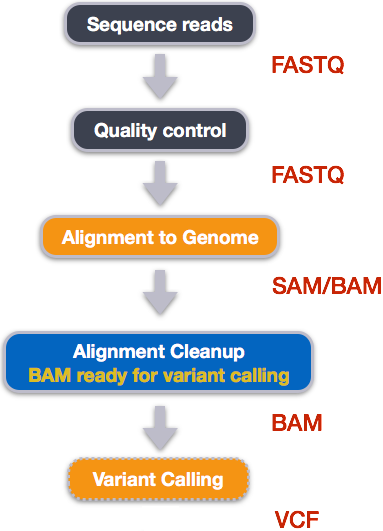
Alignment to a reference genome
We have already trimmed our reads so now the next step is alignment of our quality reads to the reference genome.
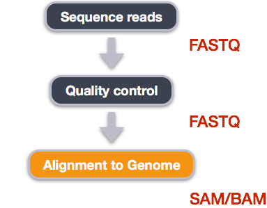
We perform read alignment or mapping to determine where in the genome our reads originated from. There are a number of tools to choose from and, while there is no gold standard, there are some tools that are better suited for particular NGS analyses. We will be using the Burrows Wheeler Aligner (BWA), which is a software package for mapping low-divergent sequences against a large reference genome. The alignment process consists of two steps:
- Indexing the reference genome
- Aligning the reads to the reference genome
Setting up
First we will copy the reference genome data into our data/ directory, as well as a set of trimmed FASTQ files to work with in this lesson, and a set of untrimmed files for the next one.
$ cd /pool/genomics/username/dc_workshop
$ cp -r /data/genomics/workshops/data_carpentry_genomics/dc_sampledata_lite/ref_genome/ data/
$ cp -r /data/genomics/workshops/data_carpentry_genomics/dc_sampledata_lite/trimmed_fastq_small/ data/
You will also need to create directories for the results that will be generated as part of this workflow. We can do this in a single
line of code because mkdir can accept multiple new directory
names as input.
$ mkdir -p results/sai results/sam results/bam results/bcf results/vcf
Loading modules
It’s worth noting here that all of the software we are using for this workshop has been pre-installed on Hydra. You’ll need to load the software modules first. Today we are working on the interactive node (that you called using qrsh), but you could also submit jobs using qsub.
Index the reference genome
Our first step is to index the reference genome for use by BWA. This helps speed up our alignment.
To Index or Not To Index
Indexing the reference only has to be run once. The only reason you would want to create a new index is if you are working with a different reference
genome or you are using a different tool for alignment.
$ module load bioinformatics/bwa
$ bwa index data/ref_genome/ecoli_rel606.fasta
While the index is created, you will see output something like this:
[bwa_index] Pack FASTA... 0.07 sec
[bwa_index] Construct BWT for the packed sequence...
[bwa_index] 1.83 seconds elapse.
[bwa_index] Update BWT... 0.03 sec
[bwa_index] Pack forward-only FASTA... 0.05 sec
[bwa_index] Construct SA from BWT and Occ... 0.64 sec
[main] Version: 0.7.17-r1188
[main] CMD: bwa index data/ref_genome/ecoli_rel606.fasta
[main] Real time: 2.801 sec; CPU: 2.627 sec
Align reads to reference genome
The alignment process consists of choosing an appropriate reference genome to map our reads against and then deciding on an aligner. BWA consists of three algorithms: BWA-backtrack, BWA-SW and BWA-MEM. The first algorithm is designed for Illumina sequence reads up to 100bp, while the other two are for sequences ranging from 70bp to 1Mbp. BWA-MEM and BWA-SW share similar features such as long-read support and split alignment, but BWA-MEM, which is the latest, is generally recommended for high-quality queries as it is faster and more accurate.
Since we are working with short reads we will be using BWA-backtrack. The general usage for BWA-backtrack is:
$ bwa aln ref_genome.fasta input_file.fastq > output_file.sai
This will create a .sai file which is an intermediate file containing the suffix array indexes.
Have a look at the bwa options page. While we are running bwa with the default parameters here, your use case might require a change of parameters. NOTE: Always read the manual page for any tool before using and make sure the options you use are appropriate for your data.
We’re going to start by aligning the reads from just one of the
samples in our dataset (SRR097977.fastq). Later, we’ll be
iterating this whole process on all of our sample files.
$ bwa aln data/ref_genome/ecoli_rel606.fasta data/trimmed_fastq_small/SRR097977.fastq_trim.fastq > results/sai/SRR097977.aligned.sai
You will see output that starts like this:
[bwa_aln] 17bp reads: max_diff = 2
[bwa_aln] 38bp reads: max_diff = 3
[bwa_aln] 64bp reads: max_diff = 4
[bwa_aln] 93bp reads: max_diff = 5
[bwa_aln] 124bp reads: max_diff = 6
[bwa_aln] 157bp reads: max_diff = 7
[bwa_aln] 190bp reads: max_diff = 8
[bwa_aln] 225bp reads: max_diff = 9
[bwa_aln_core] calculate SA coordinate... 8.56 sec
Alignment cleanup
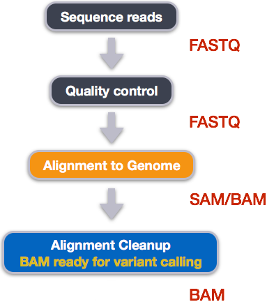
Post-alignment processing of the alignment file includes:
- Converting output SAI alignment file to a BAM file
- Sorting the BAM file by coordinate
Convert the format of the alignment to SAM/BAM
The SAI file is not a standard alignment output file and will need to be converted into a SAM file before we can do any downstream processing.
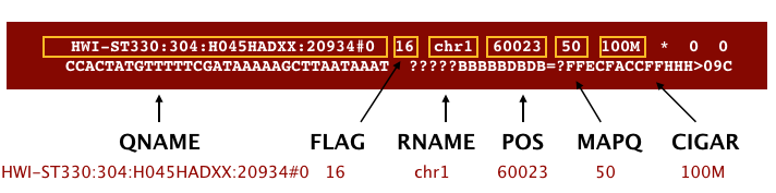
SAM/BAM format
The SAM file, is a tab-delimited text file that contains information for each individual read and its alignment to the genome. While we do not have time to go in detail of the features of the SAM format, the paper by Heng Li et al. provides a lot more detail on the specification.
The compressed binary version of SAM is called a BAM file. We use this version to reduce size and to allow for indexing, which enables efficient random access of the data contained within the file.
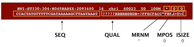
The file begins with a header, which is optional. The header is used to describe source of data, reference sequence, method of alignment, etc., this will change depending on the aligner being used. Following the header is the alignment section. Each line that follows corresponds to alignment information for a single read. Each alignment line has 11 mandatory fields for essential mapping information and a variable number of other fields for aligner specific information. An example entry from a SAM file is displayed below with the different fields highlighted.
Better viewing of tab delminated files
Tab seperated files can sometimes be hard to view in the terminal. You may find that the headers don’t line up with columns and that long lines wrap to the next line. Try using
less -S -x10 filenameto view the file.-Scauses less to not wrap long lines, use the left and right arrow keys to see more of the line.-x10expands how many spaces each tab displays as to 10 character which will help the columns to line up. You can try larger values for x to make the columns wider.
First we will use the bwa samse command to convert the .sai file to SAM format. The usage for bwa samse is
$ bwa samse ref_genome.fasta input_file.sai input_file.fastq > output_file.sam
The code in our case will look like:
$ bwa samse data/ref_genome/ecoli_rel606.fasta \
        results/sai/SRR097977.aligned.sai \
        data/trimmed_fastq_small/SRR097977.fastq_trim.fastq > \
        results/sam/SRR097977.aligned.sam
Your output will start out something like this:
bwa_aln_core] convert to sequence coordinate... 1.03 sec
[bwa_aln_core] refine gapped alignments... 0.17 sec
[bwa_aln_core] print alignments... 0.65 sec
[bwa_aln_core] 262144 sequences have been processed.
[bwa_aln_core] convert to sequence coordinate... 0.58 sec
[bwa_aln_core] refine gapped alignments... 0.09 sec
[bwa_aln_core] print alignments... 0.37 sec
[bwa_aln_core] 406070 sequences have been processed.
Multiple line commands
When typing a long command into your terminal, you can use the
\character to separate code chunks onto separate lines. This can make your code more readable.
Next we convert the SAM file to BAM format for use by downstream tools. We use the samtools program with the view command and tell this command that the input is in SAM format (-S) and to output BAM format (-b):
$ module load bioinformatics/samtools
$ samtools view -S -b results/sam/SRR097977.aligned.sam > results/bam/SRR097977.aligned.bam
Sort BAM file by coordinates
Next we sort the BAM file using the sort command from samtools. Note that as second parameter, we give the filename of the desired output file without the .bam part:
$ samtools sort results/bam/SRR097977.aligned.bam > results/bam/SRR097977.aligned.sorted.bam
More Than One Way to . . . sort a SAM/BAM File
SAM/BAM files can be sorted in multiple ways, e.g. by location of alignment on the chromosome, by read name, etc. It is important to be aware that different alignment tools will output differently sorted SAM/BAM, and different downstream tools require differently sorted alignment files as input.*
Variant calling
A variant call is a conclusion that there is a nucleotide difference vs. some reference at a given position in an individual genome
or transcriptome, often referred to as a Single Nucleotide Polymorphism (SNP). The call is usually accompanied by an estimate of
variant frequency and some measure of confidence. Similar to other steps in this workflow, there are number of tools available for
variant calling. In this workshop we will be using bcftools, but there are a few things we need to do before actually calling the
variants.
Step 1: Calculate the read coverage of positions in the genome
Do the first pass on variant calling by counting read coverage with samtools mpileup:
$ samtools mpileup -g -f data/ref_genome/ecoli_rel606.fasta \
            results/bam/SRR097977.aligned.sorted.bam > results/bcf/SRR097977_raw.bcf
[mpileup] 1 samples in 1 input files
<mpileup> Set max per-file depth to 8000
We have now generated a file with coverage information for every base. To identify variants, we now will use a different tool from the samtools suite called bcftools.
Step 2: Detect the single nucleotide polymorphisms (SNPs)
Identify SNPs using bcftools:
$ module load bioinformatics/bcftools
$ bcftools call -vm -O b results/bcf/SRR097977_raw.bcf > results/bcf/SRR097977_variants.bcf
Step 3: Filter and report the SNP variants in variant calling format (VCF)
Filter the SNPs for the final output in VCF format, using vcfutils.pl:
$ bcftools view results/bcf/SRR097977_variants.bcf | \
  vcfutils.pl varFilter - > results/vcf/SRR097977_final_variants.vcf
bcftools view converts the binary format of bcf files into human readable format (tab-delimited) for vcfutils.pl to perform
the filtering. Note that the output is in VCF format, which is a text format.
Explore the VCF format:
$ less results/vcf/SRR097977_final_variants.vcf
You will see the header (which describes the format), the time and date the file was created, the version of bcftools that was used, the command line parameters used, and some additional information:
##fileformat=VCFv4.2
##FILTER=<ID=PASS,Description="All filters passed">
##samtoolsVersion=1.3.1+htslib-1.3.1
##samtoolsCommand=samtools mpileup -g -f data/ref_genome/ecoli_rel606.fasta results/bam/SRR097977.aligned.sorted.bam
##reference=file://data/ref_genome/ecoli_rel606.fasta
##contig=<ID=NC_012967.1,length=4629812>
##ALT=<ID=*,Description="Represents allele(s) other than observed.">
##INFO=<ID=INDEL,Number=0,Type=Flag,Description="Indicates that the variant is an INDEL.">
##INFO=<ID=IDV,Number=1,Type=Integer,Description="Maximum number of reads supporting an indel">
##INFO=<ID=IMF,Number=1,Type=Float,Description="Maximum fraction of reads supporting an indel">
##INFO=<ID=DP,Number=1,Type=Integer,Description="Raw read depth">
##INFO=<ID=VDB,Number=1,Type=Float,Description="Variant Distance Bias for filtering splice-site artefacts in RNA-seq data (bigger is better)",Version="3">
##INFO=<ID=RPB,Number=1,Type=Float,Description="Mann-Whitney U test of Read Position Bias (bigger is better)">
.
.
.
.
##FORMAT=<ID=PL,Number=G,Type=Integer,Description="List of Phred-scaled genotype likelihoods">
##FORMAT=<ID=GT,Number=1,Type=String,Description="Genotype">
##INFO=<ID=ICB,Number=1,Type=Float,Description="Inbreeding Coefficient Binomial test (bigger is better)">
##INFO=<ID=HOB,Number=1,Type=Float,Description="Bias in the number of HOMs number (smaller is better)">
##INFO=<ID=AC,Number=A,Type=Integer,Description="Allele count in genotypes for each ALT allele, in the same order as listed">
##INFO=<ID=AN,Number=1,Type=Integer,Description="Total number of alleles in called genotypes">
##INFO=<ID=DP4,Number=4,Type=Integer,Description="Number of high-quality ref-forward , ref-reverse, alt-forward and alt-reverse bases">
##INFO=<ID=MQ,Number=1,Type=Integer,Description="Average mapping quality">
Followed by information on each of the variations observed:
#CHROM  POS     ID      REF     ALT     QUAL    FILTER  INFO    FORMAT  results/bam/SRR097977.aligned.sorted.bam
NC_012967.1     9972    .       T       G       66      .       DP=3;VDB=0.220755;SGB=-0.511536;MQSB=1;MQ0F=0;AC=2;AN=2;DP4=0,0,1,2;MQ=37       GT:PL   1/1:96,9,0
NC_012967.1     10563   .       G       A       24.4299 .       DP=2;VDB=0.36;SGB=-0.453602;MQ0F=0;AC=2;AN=2;DP4=0,0,0,2;MQ=37  GT:PL   1/1:54,6,0
NC_012967.1     81158   .       A       C       148     .       DP=8;VDB=0.250641;SGB=-0.636426;MQSB=1.01283;MQ0F=0;AC=2;AN=2;DP4=0,0,4,3;MQ=37 GT:PL   1/1:178,21,0
NC_012967.1     139812  .       G       T       8.07754 .       DP=4;VDB=0.56;SGB=-0.453602;RPB=1;MQB=1;MQSB=1;BQB=0.25;MQ0F=0;ICB=1;HOB=0.5;AC=1;AN=2;DP4=0,2,1,1;MQ=37        GT:PL   0/1:40,0,49
NC_012967.1     216480  .       C       T       62      .       DP=4;VDB=0.235765;SGB=-0.511536;MQSB=1;MQ0F=0;AC=2;AN=2;DP4=0,0,1,2;MQ=37       GT:PL   1/1:92,9,0
NC_012967.1     247796  .       T       C       58      .       DP=3;VDB=0.102722;SGB=-0.511536;MQSB=1;MQ0F=0;AC=2;AN=2;DP4=0,0,1,2;MQ=33       GT:PL   1/1:88,9,0
NC_012967.1     281923  .       G       T       38.415  .       DP=2;VDB=0.06;SGB=-0.453602;MQSB=1;MQ0F=0;AC=2;AN=2;DP4=0,0,1,1;MQ=37   GT:PL   1/1:68,6,0
This is a lot of information, so let’s take some time to make sure we understand our output.
The first few columns represent the information we have about a predicted variation.
| column | info |
|---|---|
| CHROM | contig location where the variation occurs |
| POS | position within the contig where the variation occurs |
| ID | a . until we add annotation information |
| REF | reference genotype (forward strand) |
| ALT | sample genotype (forward strand) |
| QUAL | Phred-scaled probablity that the observed variant exists at this site (higher is better) |
| FILTER | a . if no quality filters have been applied, PASS if a filter is passed, or the name of the filters this variant failed |
In an ideal world, the information in the QUAL column would be all we needed to filter out bad variant calls.
However, in reality we need to filter on multiple other metrics.
The last two columns contain the genotypes and can be tricky to decode.
| column | info |
|---|---|
| FORMAT | lists in order the metrics presented in the final column |
| results | lists the values associated with those metrics in order |
For our file, the metrics presented are DP:VDB:SGB:MQSB:MQOF:AC:AN:DP4:MQ:GT:PL.
| metric | definition |
|---|---|
| GT | the genotype of this sample which for a diploid genome is encoded with a 0 for the REF allele, 1 for the first ALT allele, 2 for the second and so on. So 0/0 means homozygous reference, 0/1 is heterozygous, and 1/1 is homozygous for the alternate allele. For a diploid organism, the GT field indicates the two alleles carried by the sample, encoded by a 0 for the REF allele, 1 for the first ALT allele, 2 for the second ALT allele, etc. |
| PL | the likelihoods of the given genotypes |
| GQ | the Phred-scaled confidence for the genotype |
| AD, DP | the depth per allele by sample and coverage |
The Broad Institute’s VCF guide is an excellent place to learn more about VCF file format.
Exercise
Use the
grep,cut, andlesscommands you’ve learned to extract thePOSandQUALcolumns from your output file (without the header lines). What is the position of the first variant to be called with aQUALvalue of less than 4?Solution
$ cut results/vcf/SRR097977_final_variants.vcf -f 6,2 | grep -v "##" | lessPOS QUAL 9972 66 10563 24.429 81158 148 139812 8.07754 216480 62 247796 58 281923 38.415 . . . 788403 4.97012 911613 3.88886Position 911613 has a score of 3.88886.
Assess the alignment (visualization) - optional step
It is often instructive to look at your data in a genome browser. Visualisation will allow you to get a “feel” for the data, as well as detecting abnormalities and problems. Also, exploring the data in such a way may give you ideas for further analyses. As such, visualization tools are useful for exploratory analysis. In this lesson we will describe two different tools for visualisation; a light-weight command-line based one and the Broad Institute’s Integrative Genomics Viewer (IGV) which requires software installation and transfer of files.
In order for us to visualize the alignment files, we will need to index the BAM file using samtools:
$ samtools index results/bam/SRR097977.aligned.sorted.bam
Viewing with tview
Samtools implements a very simple text alignment viewer based on the GNU
ncurses library, called tview. This alignment viewer works with short indels and shows MAQ consensus.
It uses different colors to display mapping quality or base quality, subjected to users’ choice. Samtools viewer is known to work with an 130 GB alignment swiftly. Due to its text interface, displaying alignments over network is also very fast.
In order to visualize our mapped reads we use tview, giving it the sorted bam file and the reference file:
$ samtools tview results/bam/SRR097977.aligned.sorted.bam data/ref_genome/ecoli_rel606.fasta
1         11        21        31        41        51        61        71        81        91        101       111       121
AGCTTTTCATTCTGACTGCAACGGGCAATATGTCTCTGTGTGGATTAAAAAAAGAGTGTCTGATAGCAGCTTCTGAACTGGTTACCTGCCGTGAGTAAATTAAAATTTTATTGACTTAGGTCACTAAATAC
..................................................................................................................................
,,,,,,,,,,,,,,,,,,,,,,,,,,,,,,,,,,,, ..................N................. ,,,,,,,,,,,,,,,,,,,,,,,,,,,,,,,,........................
,,,,,,,,,,,,,,,,,,,,,,,,,,,,,,,,,,, ..................N................. ,,,,,,,,,,,,,,,,,,,,,,,,,,,.............................
...................................,g,,,,,,,,,,,,,,,,,,,,,,,,,,,,,,,,,  ....................................   ................
,,,,,,,,,,,,,,,,,,,,,,,,,,,,,,,,,,,....................................   ....................................      ,,,,,,,,,,
,,,,,,,,,,,,,,,,,,,,,,,,,,,,,,,,,,,,  ....................................  ,,a,,,,,,,,,,,,,,,,,,,,,,,,,,,,,     .......
,,,,,,,,,,,,,,,,,,,,,,,,,,,,,,, .............................  ,,,,,,,,,,,,,,,,,g,,,,,    ,,,,,,,,,,,,,,,,,,,,,,,,,,,,
,,,,,,,,,,,,,,,,,,,,,,,,,,,,,,,,,,,  ...........................T.......   ,,,,,,,,,,,,,,,,,,,,,,,c,          ......
......................... ................................   ,g,,,,,,,,,,,,,,,,,,,      ...........................
,,,,,,,,,,,,,,,,,,,,, ,,,,,,,,,,,,,,,,,,,,,,,,,,,,,,, ,,,,,,,,,,,,,,,,,,,,,,,,,,,       ..........................
,,,,,,,,,,,,,,,,,,,,,,,,,,,,,,,,,,,   ................................T..  ..............................   ,,,,,,
...........................       ,,,,,,g,,,,,,,,,,,,,,,,,   ....................................         ,,,,,,
,,,,,,,,,,,,,,,,,,,,,,,,,, ....................................  ...................................        ....
....................................  ........................  ,,,,,,,,,,,,,,,,,,,,,,,,,,,,,,,,,,,,      ....
,,,,,,,,,,,,,,,,,,,,,,,,,,,,,,,,,,,,   ,,,,,,,,,,,,,,,,,,,,,,,,,,,,,,,,,,,,  ,,,,,,,,,,,,,,,,,,,,,,,,,,,,,,,,,
........................            .................................. .............................     ....
,,,,,,,,,,,,,,,,,,,,,,,,,,,,,,,,,,,,   ....................................        ..........................
...............................       ,,,,,,,,,,,,,,,,,,,,,,,,,,,,,,,, ....................................
...................................  ,,,,,,,,,,,,,,,,,,,,,,,,,,,,,,,,  ,,,,,,,,,,,,,,,,,,,,,,,,,,,,,,,,,,,
,,,,,,,,,,,,,,,,,,,,,,,,,,,,,,,,,,,, ,,,,,,,,,,,,,,,,,,,,,,,,,,,,,,,,,,  ..................................
.................................... ,,,,,,,,,,,,,,,,,,a,,,,,,,,,,,,,,,,,        ,,,,,,,,,,,,,,,,,,,,,,,,,
,,,,,,,,,,,,,,,,,,,,,,,,,,,,,,,,,,,  ............................ ,,,,,,,,,,,,,,,,,,,,,,,,,,,,,,,,,,,,
The first line of output shows the genome coordinates in our reference genome. The second line shows the reference
genome sequence. The third lines shows the consensus sequence determined from the sequence reads. A . indicates
a match to the reference sequence, so we can see that the consensus from our sample matches the reference in most
locations. That is good! If that wasn’t the case, we should probably reconsider our choice of reference.
Below the horizontal line, we can see all of the reads in our sample aligned with the reference genome. Only
positions where the called base differs from the reference are shown. You can use the arrow keys on your keyboard
to scroll or type ? for a help menu. Type Ctrl^C to exit tview.
Viewing with IGV
IGV is a stand-alone browser, which has the advantage of being installed locally and providing fast access. Web-based genome browsers, like Ensembl or the UCSC browser, are slower, but provide more functionality. They not only allow for more polished and flexible visualisation, but also provide easy access to a wealth of annotations and external data sources. This makes it straightforward to relate your data with information about repeat regions, known genes, epigenetic features or areas of cross-species conservation, to name just a few.
In order to use IGV, we will need to transfer some files to our local machine. We know how to do this with scp.
Open a new tab in your terminal window and create a new folder. We’ll put this folder on our Desktop for
demonstration purposes, but in general you should avoide proliferating folders and files on your Desktop and
instead organize files within a directory structure like we’ve been using in our dc_workshop directory.
$ mkdir ~/Desktop/files_for_igv
$ cd ~/Desktop/files_for_igv
Now we will transfer our files to that new directory. The commands to scp always go in the terminal window that is connected to your local computer (not to Hydra).
$ scp username@hydra-login01.si.edu:/pool/genomics/username/dc_workshop/results/bam/SRR097977.aligned.sorted.bam ~/Desktop/files_for_igv
$ scp username@hydra-login01.si.edu:/pool/genomics/username/dc_workshop/results/bam/SRR097977.aligned.sorted.bam.bai ~/Desktop/files_for_igv
$ scp username@hydra-login01.si.edu:/pool/genomics/username/dc_workshop/data/ref_genome/ecoli_rel606.fasta ~/Desktop/files_for_igv
$ scp username@hydra-login01.si.edu:/pool/genomics/username/dc_workshop/results/vcf/SRR097977_final_variants.vcf ~/Desktop/files_for_igv
You will need to type your Hydra password each time you call scp.
Alternatively, you can copy everything using one command, and add the password only once. Each path/file is separated by a space and all files to be copied are delimited by a a single quote (‘):
$ scp username@hydra-login01.si.edu:'/scratch/genomics/username/dc_workshop/results/bam/SRR097977.aligned.sorted.bam \
/scratch/genomics/username/dc_workshop/results/bam/SRR097977.aligned.sorted.bam.bai \
/scratch/genomics/username/dc_workshop/data/ref_genome/ecoli_rel606.fasta \ /scratch/genomics/username/dc_workshop/results/vcf/SRR097977_final_variants.vcf' \
~/Desktop/files_for_igv/
Next we need to open the IGV software. If you haven’t done so already, you can download IGV from the Broad Institute’s software page, double-click the .zip file
to unzip it, and then drag the program into your Applications folder.
- Open IGV.
- Load our reference genome file (
ecoli_rel606.fasta) into IGV using the “Load Genomes from File…“ option under the “Genomes” pull-down menu. - Load our BAM file (
SRR097977.aligned.sorted.bam) using the “Load from File…“ option under the “File” pull-down menu. - Do the same with our VCF file (
SRR097977_final_variants.vcf).
Your IGV browser should look like the screenshot below:
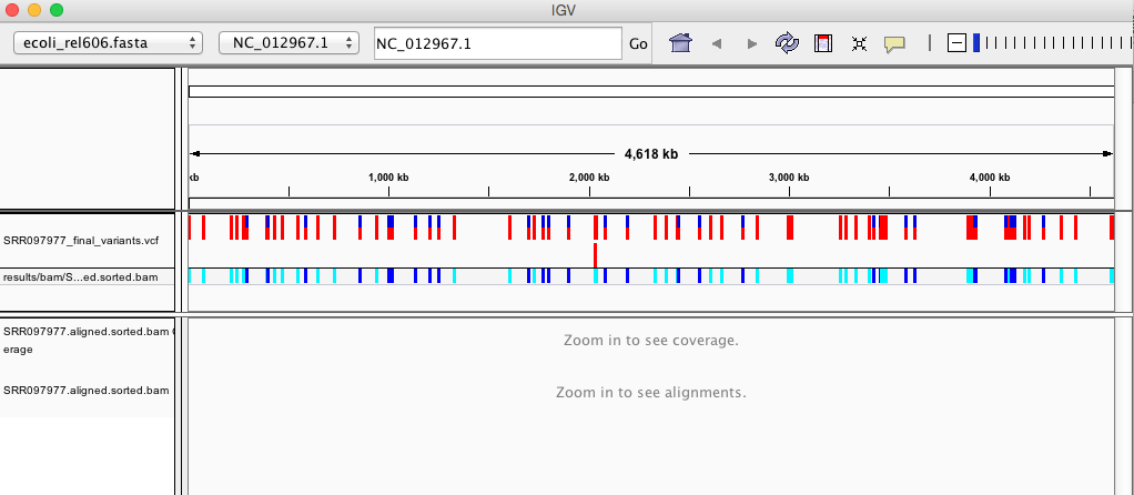
There should be two tracks: one coresponding to our BAM file and the other for our VCF file.
In the VCF track, each bar across the top of the plot shows the allele fraction for a single locus. The second bar shows the genotypes for each locus in each sample. We only have one sample called here so we only see a single line. Dark blue = heterozygous, Cyan = homozygous variant, Grey = reference. Filtered entries are transparent.
Zoom in to inspect variants you see in your filtered VCF file to become more familiar with IGV. See how quality information corresponds to alignment information at those loci. Use this website and the links therein to understand how IGV colors the alignments.
Now that we’ve run through our workflow for a single sample, we want to repeat this workflow for our other five samples. However, we don’t want to type each of these individual steps again five more times. That would be very time consuming and error-prone, and would become impossible as we gathered more and more samples. Luckily, we already know the tools we need to use to automate this workflow and run it on as many files as we want using a single line of code. Those tools are: wildcards, for loops, and bash scripts. We’ll use all three in the next lesson.
Key Points
Bioinformatics command line tools are collections of commands that can be used to carry out bioinformatics analyses.
To use most powerful bioinformatics tools, you’ll need to use the command line.
There are many different file formats for storing genomics data. It’s important to understand these file formats and know how to convert among them.